

Yale Model vs. Probabilistic Models
When institutional and private investors commit capital to illiquid alternatives—private equity, venture capital, infrastructure, and private credit—they face a distinct “cash-flow pacing” challenge: the timing of capital calls and distributions is unpredictable, making it difficult to maintain target allocations without either running short of liquidity or holding too much idle cash.
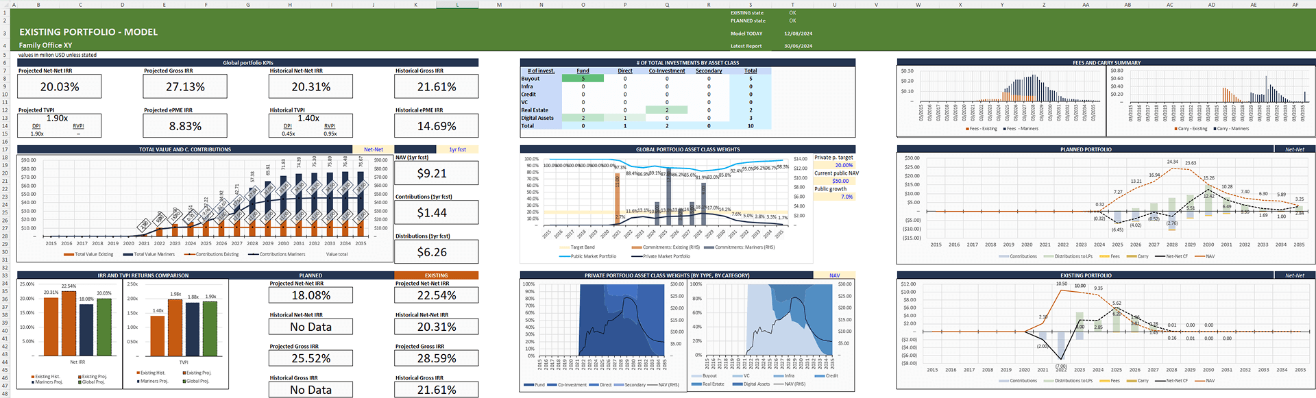
Financial modelers often turn to in-house Excel models to forecast these cash flows and guide new commitments. Two major approaches to modeling these cash flows are deterministic and probabilistic, each with its own trade-offs:
• The traditional deterministic approach (the “Yale Model”): Relies on average industry assumptions, offering simplicity and ease of use. It is quick to stress-test but may not capture the full range of possible outcomes or swiftly adapt to market shifts.
• New, often proprietary probabilistic approaches: Generates a distribution of possible paths, capturing best- and worst-case liquidity scenarios. While powerful, it requires more data, complexity, and specialized skills to build and maintain.
Those who decide to build a traditional Yale Model type of Cash Flow Pacing model, below are a few considerations and decisions that will help you to ensure your Excel model is robust, flexible, and aligned with your organization’s goals.
1. Forecasting and Reporting Capabilities
- Forecast Only
- Report of Actuals Only
- Rolling Forecast Updated Based on Actuals
Your model’s forecasting and reporting capabilities define its overall functionality. At one end of the spectrum, a forecast-only model suits strategic, long-term portfolio allocation decisions—ideal when the emphasis is on high-level projections and scenario planning. On the other end, a report of actuals only approach serves well for historical performance evaluation, where detailed tracking of realized cash flows is essential.
For many applications, however, a hybrid model that updates forecasts based on actuals is the optimal choice. This dynamic approach allows for a rolling forecast that adjusts to deviations in contributions, distributions, or fees. Moreover, you will likely like to build decision pathways into your model to handle scenarios where actuals deviate from forecasts—should contributions accelerate, slow down, or should fund lifetimes extend? Incorporating these pathways improves the ability for confident decision making during market stress or unexpected asset behavior.
2. Model Periodicity
- Annual
- Quarterly
Annual models are typically sufficient for high-level strategic planning, offering a bird’s-eye view of the portfolio’s evolution. However, quarterly models might be more suitable for tracking of actuals, monitoring short-term performance or more granular estimates for cash-flow management.
A model that must both display and update based on actuals will benefit from a periodicity that aligns with how frequently new data becomes available, thereby reducing discrepancies and improving decision-making accuracy.
3. Fees, Carry & Gross / Net View
Model with Management Fees and Carry or Advisor Fees
- Net Only Model
- Model with Management Fees, Carry, Advisor Fees, Expenses
Incorporating management fees, fund expenses, carry, or even advisor fees into your model is essential for realistic gross-to-net performance analysis. When projecting future cash flows or evaluating historical performance, toggling between a gross, net, or net-net basis can yield valuable insights.
An important technical consideration is avoiding circularity within the model. When management fees are calculated based on the same cash flows they affect, it can lead to complex dependencies. Structuring your model to clearly segregate fee calculations or simplifying the fee estimates can help avoid cirtularities in the model.
4. Waterfall Modeling
The waterfall levels you include — be it current income, carried interest, GP catch-up, or other fund-specific allocations — directly impact the accuracy of your gross/net calculations. Tailoring the waterfall to match the specific conditions of your investments not only improves the model’s explanatory power but also enables a more nuanced understanding of value creation in time.
5. Structure and Level of Detail of Inputs of Actuals
- Historical Time-Series Data (Calls, Distributions, Fees, NAVs)
- Basic Snapshot at one point in time (last period cumulative calls, distributions, NAV)
When deciding on the level of detail for your inputs, balance the need for precision against the practicality of data collection. A full historical time-series approach obviously provides a better picture of historical development (as well as some waterfall critical data-points, such as preferred return balance). However, in scenarios where deep detail is neither available nor necessary, a basic snapshot of the most recent cumulative figures can simplify the user’s workload and still offer informative future estimates.

6. Cash Flow Pacing Inputs
Contributions:
- Takahashi-Alexander Model (% of Unfunded per Year)
- Cumulative Contributions Year-by-Year
- Historical Experience or Commercial Data Sets
Distributions:
- Takahashi-Alexander Model
- Possibility of Bullet Repayments or distributions with "right-skewed" distributions (direct buyout exits etc)
The method you choose for pacing cash flows can significantly influence the model’s predictive power. For contributions, the Takahashi-Alexander style provides a structured framework that many practitioners favor for its balance of historical data and market-based assumptions. Alternatively, inputting cumulative contributions might provide better control to more closely match historical or forecasted developments. Relying on commercial data sets or historical experience always offer a statistically grounded approach, although such data come at cost.
For distributions, understanding the nature of the underlying assets is critical. A Takahashi-Alexander approach might work well for certain asset classes, but other scenarios—such as those involving bullet repayments or bell-shaped repayment curves typical in buyouts—require tailored pacing inputs to capture the nuances of cash flow timing and magnitude.
7. Scalability and Maintainability of the Model
- Fixed number of potential commitments
- Flexible model with "unlimited" commitments
The scalability of your model is crucial. A single commitment might only need a few rows of calculations, but if you’re modeling an entire portfolio with fee structures, waterfall detail, actuals and projected time-series and so on, each commitment could require anywhere from 200 to 400 rows in your model. With 5 asset classes with commitments projected for 15 years for each, you will easily get into low tens of thousands of rows.
Therefore, planning for scalability—from 10 to 100 or even more commitments—is essential for maintaining performance and usability, especially in an institutional setting where portfolio sizes can be substantial.
Decide what your needs are and where you need to make your model flexible.
8. Classification of Commitments
• Classification by asset class, strategy, region, status (realized/unrealized), sponsor, etc.
Finally, how you classify commitments within your model can provide critical insights and enable more sophisticated analysis. Classifications such as asset class, investment strategy, geographic region, performance status, and sponsor identity allow you to slice and dice the data for deeper portfolio analytics. This granularity can inform decisions on rebalancing, risk management, and targeted strategy adjustments.
By integrating classification into your model, you can create either fixed or advanced dynamic reports and dashboards that help you better understand forecasted portfolio exposures in time, projected performance and other metrics and better optimize planned commitments. This level of detail is particularly valuable in a multi-faceted portfolio where different commitments may behave very differently under various market conditions.